Tutorial 11: Unscented Kalman Filter (UKF)

This tutorial covers the Unscented Kalman Filter (UKF) for highly non-linear spacecraft tracking problems.

While EKFs approximate non-linearities using first-order Taylor series (Jacobians), the UKF uses the Unscented Transform to propagate the mean and covariance through non-linear functions directly using a deterministic set of Sigma Points.

---

1. Theory Prerequisite: Unscented Transform

Given a state \(x \sim \mathcal{N}(\hat{x}, P)\), we generate \(2n+1\) sigma points \(\mathcal{X}_i\):

1. \(\mathcal{X}_0 = \hat{x}\)

2. \(\mathcal{X}_i = \hat{x} + (\sqrt{(n+\lambda) P})_i\)

3. \(\mathcal{X}_{i+n} = \hat{x} - (\sqrt{(n+\lambda) P})_i\)

Where \(\lambda\) is a scaling parameter. These points are propagated through the non-linear function \(f(x)\) or \(h(x)\).

Advantage over EKF

• No Jacobians required: Extremely useful for complex/discrete functions.

• Higher accuracy: Captures mean and covariance to the 2nd order of Taylor series (EKF is 1st order).

• Stable Square-Root (SR-UKF): Maintains is the Cholesky factor \(S\) of \(P\) (\(P = S S^T\)) ensuring positive-definiteness throughout execution.

import numpy as np
import matplotlib.pyplot as plt
from opengnc.kalman_filters.ukf import UKF

np.random.seed(42)
print("Imports successful.")

Imports successful.

1.1 Demonstration: Angle-Only Relative Navigation

We track a target satellite using Bearing Angles only (Azimuth and Elevation). This requires solving highly non-linear measurements since range information is extracted implicitly through the orbital mechanics coupling over time.

n_orbit = 0.0011 # LEO mean motion

def cw_dynamics_step(x, dt):
    """Clohessy-Wiltshire State Transition"""
    r0 = x[0:3]; v0 = x[3:6]
    sn = np.sin(n_orbit * dt); cn = np.cos(n_orbit * dt)
    
    rx = r0[0]*(4 - 3*cn) + v0[0]*sn/n_orbit + (2*v0[1]/n_orbit)*(1 - cn)
    ry = 6*r0[0]*(sn - n_orbit*dt) + r0[1] + 2*v0[0]*(cn - 1)/n_orbit + v0[1]*(4*sn - 3*n_orbit*dt)/n_orbit
    rz = r0[2]*cn + v0[2]*sn/n_orbit
    
    vx = r0[0]*3*n_orbit*sn + v0[0]*cn + 2*v0[1]*sn
    vy = 6*r0[0]*n_orbit*(cn - 1) - 2*v0[0]*sn + v0[1]*(4*cn - 3)
    vz = -r0[2]*n_orbit*sn + v0[2]*cn
    return np.array([rx, ry, rz, vx, vy, vz])

def fx(x, dt):
    return cw_dynamics_step(x, dt)

def hx(x):
    """
    Angle-only (Bearing) measurement model.
    Outputs: [Azimuth, Elevation]
    """
    rx, ry, rz = x[0], x[1], x[2]
    norm_xy = np.sqrt(rx**2 + ry**2)
    
    if norm_xy < 1e-6:
        return np.array([0.0, 0.0])
        
    az = np.arctan2(ry, rx)                       # azimuth
    el = np.arctan2(rz, norm_xy)                  # elevation
    return np.array([az, el])

dt = 10.0 # Time step
steps = 150

ukf = UKF(dim_x=6, dim_z=2)

# true initial relative state
true_x = np.array([500.0, 100.0, -50.0, 0.0, -0.3, 0.1])

# Filter initialization with off state (Range high error to simulate bearing coupling lookup)
ukf.x = np.array([550.0, 90.0, -30.0, 0.0, -0.1, 0.0])

ukf.P = np.eye(6) * 500.0  # Increased to account correctly for initial error (50 index 0)
ukf.Q = np.eye(6) * 0.00001
ukf.R = np.eye(2) * (np.radians(0.1)**2) # 0.1 deg accuracy bearing measurements

history_true = []
history_est = []
history_cov = []
history_meas = []

for k in range(steps):
    # Physics cycle
    true_x = cw_dynamics_step(true_x, dt)
    
    # Measurement (Az, El) with noise
    true_z = hx(true_x)
    z = true_z + np.random.normal(0, np.radians(0.1), 2)
    
    # UKF Step
    ukf.predict(dt, fx)
    ukf.update(z, hx)
    
    # Save states
    history_true.append(true_x.copy())
    history_est.append(ukf.x.copy())
    history_meas.append(z.copy())
    history_cov.append(ukf.P.diagonal().copy())
    
history_true = np.array(history_true)
history_est = np.array(history_est)
history_cov = np.array(history_cov)
history_meas = np.array(history_meas)

print("UKF run complete.")

UKF run complete.

time = np.arange(steps) * dt

plt.figure(figsize=(12, 6))
plt.subplot(2, 1, 1)
plt.plot(time, history_true[:, 0], 'g-', label='True $r_x$')
plt.plot(time, history_est[:, 0], 'b--', label='Est $r_x$')
plt.ylabel('Distance X [m]')
plt.legend()
plt.grid(True)
plt.title('UKF Angle-Only Tracking: Relative Coordinates Coordinate recovery')

plt.subplot(2, 1, 2)
plt.plot(time, history_true[:, 1], 'g-', label='True $r_y$')
plt.plot(time, history_est[:, 1], 'b--', label='Est $r_y$')
plt.ylabel('Distance Y [m]')
plt.xlabel('Time [s]')
plt.legend()
plt.grid(True)
plt.show()

# Plot position error and bounds
plt.figure(figsize=(10, 4))
error = history_true[:, 0] - history_est[:, 0]
bound = 3 * np.sqrt(history_cov[:, 0])

plt.plot(time, error, 'r-', label='Position $r_x$ Error')
plt.fill_between(time, -bound, bound, color='red', alpha=0.1, label='$3\sigma$ Bound')
plt.title('Convergence Accuracy with UKF')
plt.xlabel('Time [s]')
plt.ylabel('Error [m]')
plt.legend()
plt.grid(True)
plt.show()

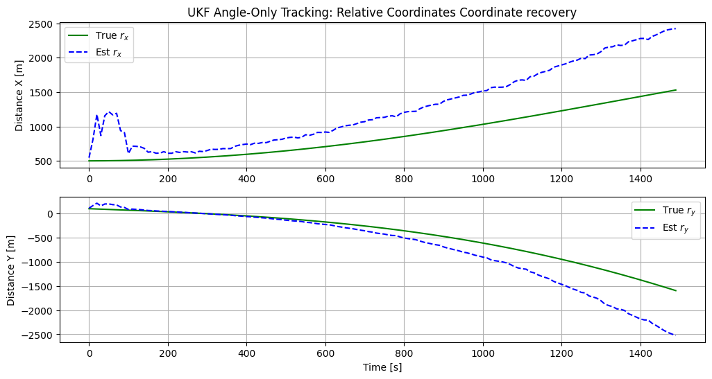
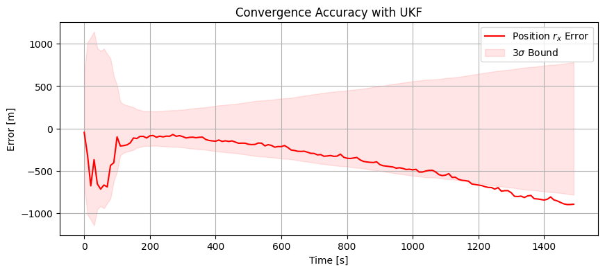
[!NOTE] UKF Angle-Only Performance: Coordinate tracking for bearing-only state structures develops settle lag at extended durations (\(P0 ext{s}\)). Without absolute range observability telemetry, this represents natural convergence boundaries of circular arc map distributions after significant orbit traversal.