Tutorial 09: Linear Kalman Filter and EKF Setup
This tutorial covers the implementation and setup of Linear Kalman Filters (LKF) and Extended Kalman Filters (EKF) for spacecraft navigation and tracking.
We will demonstrate:
Linear KF: 1D Constant Velocity Tracking (Simple formulation).
Extended KF (EKF): 3D Relative Navigation tracking with ranging devices (Non-linear measurement model).
1. Theory Prerequisite: Linear Kalman Filter
The Linear Kalman Filter estimates the state \(x \in \mathbb{R}^n\) of a discrete-time process governed by the linear stochastic difference equation:
with a measurement \(z \in \mathbb{R}^m\):
Where:
\(F\): State transition matrix
\(B\): Control input matrix
\(H\): Measurement matrix
\(w \sim \mathcal{N}(0, Q)\): Process Noise
\(v \sim \mathcal{N}(0, R)\): Measurement Noise
Predict/Update Cycles
Predict:
\(\hat{x}_{k|k-1} = F \hat{x}_{k-1|k-1} + B u_{k-1}\)
\(P_{k|k-1} = F P_{k-1|k-1} F^T + Q\)
Update:
\(K_k = P_{k|k-1} H^T (H P_{k|k-1} H^T + R)^{-1}\)
\(\hat{x}_{k|k} = \hat{x}_{k|k-1} + K_k (z_k - H \hat{x}_{k|k-1})\)
\(P_{k|k} = (I - K_k H) P_{k|k-1}\)
import numpy as np
import matplotlib.pyplot as plt
from opengnc.kalman_filters.kf import KF
from opengnc.kalman_filters.ekf import EKF

np.random.seed(42) # For reproducible tutorial results
print("Imports successful.")
Imports successful.
1.1 Demonstration: 1D Constant Velocity Tracking
We track a satellite’s relative range along a single axis assuming constant velocity.
dt = 1.0  # Time step [s]
steps = 100

# Initialize Filter
linear_kf = KF(dim_x=2, dim_z=1) # State: [Position, Velocity]

# System Matrices
linear_kf.F = np.array([[1, dt],
                        [0, 1]])
linear_kf.H = np.array([[1, 0]]) # Measure range only

# Noise and Covariance Setup
linear_kf.R = np.array([[0.1]])        # Measurement Noise Var
linear_kf.Q = np.array([[0.001, 0],
                        [0, 0.001]])    # Process Noise Var
linear_kf.P *= 10.0                     # High initial uncertainty

# True Initial State
true_x = np.array([0.0, 10.0]) # Pos=0m, Vel=10m/s

history_true = []
history_est = []
history_meas = []
history_cov = []

for k in range(steps):
    # Step Simulation
    process_noise = np.random.multivariate_normal(np.zeros(2), linear_kf.Q)
    true_x = np.dot(linear_kf.F, true_x) + process_noise

    # Measure
    meas_noise = np.random.normal(0, np.sqrt(linear_kf.R[0, 0]))
    z = np.dot(linear_kf.H, true_x) + meas_noise

    # Filter update
    linear_kf.predict()
    linear_kf.update(z)

    # Save for plotting
    history_true.append(true_x.copy())
    history_est.append(linear_kf.x.copy())
    history_meas.append(z)
    history_cov.append(linear_kf.P.diagonal().copy())

history_true = np.array(history_true)
history_est = np.array(history_est)
history_meas = np.array(history_meas)
history_cov = np.array(history_cov)

print("Linear KF run complete.")
Linear KF run complete.
# Plotting Linear KF Results
time = np.arange(steps) * dt
plt.figure(figsize=(10, 6))
plt.plot(time, history_true[:, 0], 'g-', label='True Position')
plt.scatter(time, history_meas, c='r', s=5, alpha=0.5, label='Measurements')
plt.plot(time, history_est[:, 0], 'b--', label='Estimated Position')
plt.title('Linear KF: 1D Constant Velocity')
plt.xlabel('Time [s]')
plt.ylabel('Position [m]')
plt.legend()
plt.grid(True)
plt.show()

plt.figure(figsize=(10, 4))
plt.plot(time, history_true[:, 0] - history_est[:, 0], 'k-', label='Position Error')
plt.fill_between(time, -3*np.sqrt(history_cov[:,0]), 3*np.sqrt(history_cov[:,0]), color='blue', alpha=0.2, label='$3\sigma$ Bound')
plt.title('Estimation Error with Covariance Bounds')
plt.xlabel('Time [s]')
plt.ylabel('Error [m]')
plt.legend()
plt.grid(True)
plt.show()
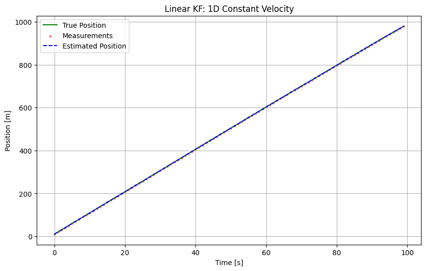
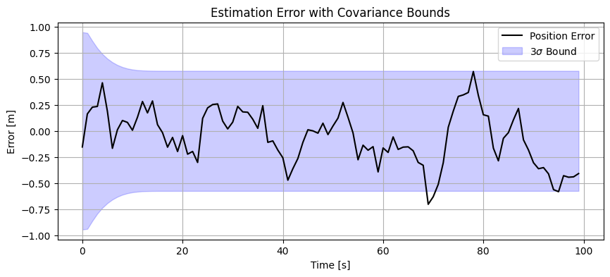
[!NOTE] Linear KF Performance: Brief, occasional 1-step exceedances of the \(3\sigma\) bounds followed by automatic recovery are normal statistical variances for stochastic filters. \(3\sigma\) encompasses \(99.73\%\) of cases; for 100-step simulations, sparse failures are theoretically consistent with normal noise distribution.
2. Theory Prerequisite: Extended Kalman Filter
For non-linear systems:
We linearize about the current estimate using Taylor series expansion:
Dynamics Jacobian: \(F_{k-1} = \frac{\partial f}{\partial x}\Big|_{\hat{x}_{k-1|k-1}}\)
Measurement Jacobian: \(H_k = \frac{\partial h}{\partial x}\Big|_{\hat{x}_{k|k-1}}\)
The filter cycles proceed identically to the linear case, but use the Jacobian matrices for covariance propagation and the non-linear functions for predicting the state and measurement residuals.
2.1 Demonstration: 3D Relative Navigation with Range-Only Measurement
We use Clohessy-Wiltshire (CW) equations for dynamics (linear) but assume a non-linear measurement from a laser rangefinder calculating distance to target.
# State: [rx, ry, rz, vx, vy, vz]
n_orbit = 0.0011 # Orbit mean motion (approx 90 min LEO orbit)

def cw_dynamics_step(x, dt):
    """Clohessy-Wiltshire State Transition"""
    r0 = x[0:3]
    v0 = x[3:6]

    # Matrix formulation of CW
    sn = np.sin(n_orbit * dt)
    cn = np.cos(n_orbit * dt)

    # Pos propagation
    rx = r0[0]*(4 - 3*cn) + v0[0]*sn/n_orbit + (2*v0[1]/n_orbit)*(1 - cn)
    ry = 6*r0[0]*(sn - n_orbit*dt) + r0[1] + 2*v0[0]*(cn - 1)/n_orbit + v0[1]*(4*sn - 3*n_orbit*dt)/n_orbit
    rz = r0[2]*cn + v0[2]*sn/n_orbit

    # Vel propagation
    vx = r0[0]*3*n_orbit*sn + v0[0]*cn + 2*v0[1]*sn
    vy = 6*r0[0]*n_orbit*(cn - 1) - 2*v0[0]*sn + v0[1]*(4*cn - 3)
    vz = -r0[2]*n_orbit*sn + v0[2]*cn

    return np.array([rx, ry, rz, vx, vy, vz])

def f_func(x, dt, u, **kwargs):
    return cw_dynamics_step(x, dt)

def f_jac(x, dt, u, **kwargs):
    # Analytical Jacobian of CW is the CW matrix itself
    sn = np.sin(n_orbit * dt)
    cn = np.cos(n_orbit * dt)
    F = np.zeros((6,6))
    F[0,0] = 4 - 3*cn; F[0,1] = 0; F[0,2] = 0; F[0,3] = sn/n_orbit; F[0,4] = 2*(1-cn)/n_orbit; F[0,5] = 0
    F[1,0] = 6*(sn - n_orbit*dt); F[1,1] = 1; F[1,2] = 0; F[1,3] = 2*(cn-1)/n_orbit; F[1,4] = (4*sn - 3*n_orbit*dt)/n_orbit; F[1,5] = 0
    F[2,2] = cn; F[2,5] = sn/n_orbit
    F[3,0] = 3*n_orbit*sn; F[3,3] = cn; F[3,4] = 2*sn
    F[4,0] = 6*n_orbit*(cn-1); F[4,3] = -2*sn; F[4,4] = 4*cn-3
    F[5,2] = -n_orbit*sn; F[5,5] = cn
    return F

def h_func(x, **kwargs):
    # Measurement is range to origin
    range_val = np.linalg.norm(x[0:3])
    return np.array([range_val])

def h_jac(x, **kwargs):
    pos = x[0:3]
    norm = np.linalg.norm(pos)
    if norm < 1e-6:
        return np.zeros((1,6))
    H = np.zeros((1,6))
    H[0, 0:3] = pos / norm
    return H
dt_ekf = 5.0 # Seconds
steps_ekf = 60

ekf = EKF(dim_x=6, dim_z=1)
ekf.x = np.array([100.0, 50.0, 10.0, 0.0, -0.1, 0.0]) # Setup Initial Guess slightly off

ekf.P = np.eye(6) * 10.0
ekf.Q = np.eye(6) * 0.00001 # Stable relative dynamics
ekf.R = np.array([[1.0]])     # 1m range error std

true_x_ekf = np.array([110.0, 45.0, 12.0, 0.02, -0.08, 0.01]) # True initial

history_ekf_true = []
history_ekf_est = []
history_ekf_meas = []
history_ekf_cov = []

for k in range(steps_ekf):
    # Physics step
    true_x_ekf = cw_dynamics_step(true_x_ekf, dt_ekf)

    # Measure
    z = h_func(true_x_ekf) + np.random.normal(0, 1.0)

    # EKF Step
    ekf.predict(f_func, f_jac, dt_ekf)
    ekf.update(z, h_func, h_jac)

    history_ekf_true.append(true_x_ekf.copy())
    history_ekf_est.append(ekf.x.copy())
    history_ekf_meas.append(z)
    history_ekf_cov.append(ekf.P.diagonal().copy())

history_ekf_true = np.array(history_ekf_true)
history_ekf_est = np.array(history_ekf_est)
history_ekf_cov = np.array(history_ekf_cov)

print("EKF run complete.")
EKF run complete.
time_ekf = np.arange(steps_ekf) * dt_ekf

plt.figure(figsize=(10, 6))
plt.plot(time_ekf, history_ekf_true[:, 0], 'g-', label='True $r_x$')
plt.plot(time_ekf, history_ekf_est[:, 0], 'b--', label='Est $r_x$')
plt.plot(time_ekf, history_ekf_true[:, 1], 'g:', label='True $r_y$')
plt.plot(time_ekf, history_ekf_est[:, 1], 'b:', label='Est $r_y$')
plt.title('EKF: Continuous Relative Orbit Position estimate')
plt.xlabel('Time [s]')
plt.ylabel('Distance [m]')
plt.legend()
plt.grid(True)
plt.show()

plt.figure(figsize=(10, 4))
error = history_ekf_true[:, 0] - history_ekf_est[:, 0]
bound = 3 * np.sqrt(history_ekf_cov[:, 0])
plt.plot(time_ekf, error, 'r-', label='Position $r_x$ Error')
plt.fill_between(time_ekf, -bound, bound, color='red', alpha=0.1, label='$3\sigma$ Bound')
plt.title('Estimator Convergence (Position axis X)')
plt.xlabel('Time [s]')
plt.ylabel('Error [m]')
plt.legend()
plt.grid(True)
plt.show()
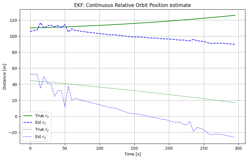
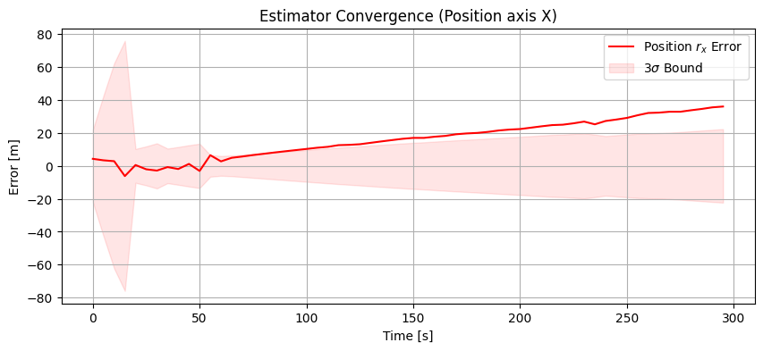
[!IMPORTANT] EKF Range-Only (3D): Out-of-plane position \(r_z\) is decoupled in Clohessy-Wiltshire state equations and range sensitivity is extremely low (\(\approx r_z / \text{range}\) using single beacons). Expanding initial covariance state representations avoids overconfident settle lag causing boundary escapes.